Try to understand what is VAE and how it run by Keras.
1 | from __future__ import absolute_import |
1 | def sampling(args): |
Choose dataset:
We will use a dataset with the shape such as this:
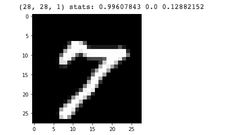
image pixels: (28, 28)
data: (N_number_of_samples, 28, 28, 1)
1 | # MNIST dataset |
Downloading data from https://storage.googleapis.com/tensorflow/tf-keras-datasets/mnist.npz 11493376/11490434 [==============================] - 0s 0us/step
11501568/11490434 [==============================] - 0s 0us/step
We loaded the MNIST dataset:
input_shape: (28, 28, 1)
x_train: (60000, 28, 28, 1)
x_test: (10000, 28, 28, 1)
1 | # Let's look at one sample: |
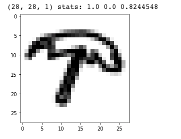
Alternative dataset - QuickDraw
We can also use the QuickDraw dataset by @Zaid Alyafeal which was used in the ML4A guide for regular AutoEncoder.
1 | !git clone https://github.com/zaidalyafeai/QuickDraw10 |
Cloning into ‘QuickDraw10’…
remote: Enumerating objects: 53, done.
remote: Total 53 (delta 0), reused 0 (delta 0), pack-reused 53
Unpacking objects: 100% (53/53), done.
1 | import numpy as np |
(80000, 28, 28, 1)
(20000, 28, 28, 1)
1 | # Let's look at one sample: |
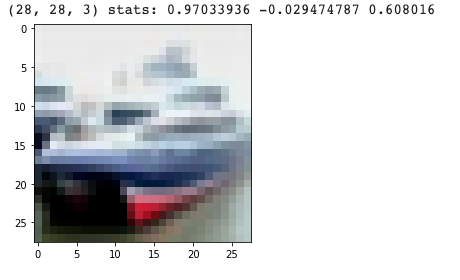
Alternative dataset - CIFAR10
1 | import keras |
Downloading data from https://www.cs.toronto.edu/~kriz/cifar-10-python.tar.gz 170500096/170498071 [==============================] - 4s 0us/step
we loaded the MNIST dataset:
input_shape: (28, 28, 1)
x_train: (50000, 32, 32, 3)
x_test: (10000, 32, 32, 3)
1 | import cv2 |
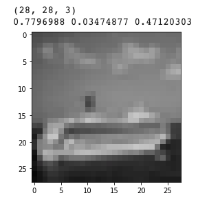
x_train: (50000, 28, 28, 3)
x_test: (10000, 28, 28, 3)
1 | x1 = x_test[1] |
Clipping input data to the valid range for imshow with RGB data ([0..1] for floats or [0..255] for integers).
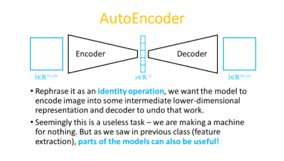
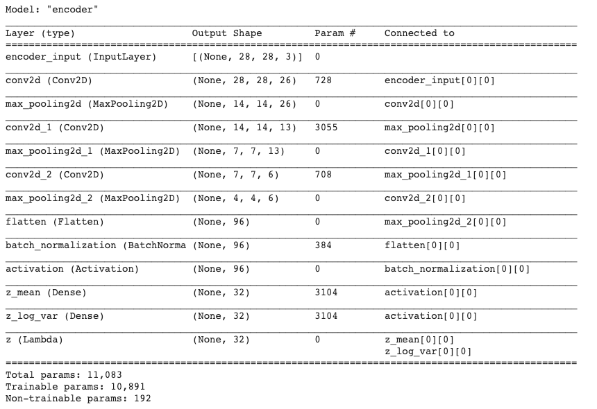
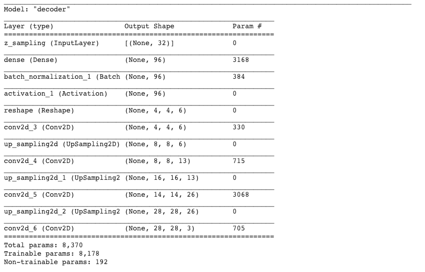
Building the model:
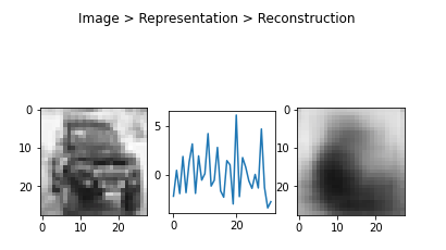
Image -> Encoder -> latent vector representation -> Decoder -> Reconstruction
Convolutional VAE
1 | # network parameters |
1 | encoder.summary() |
Continue with loaded model
1 | models = (encoder, decoder) |
1 | batch_size = 128*2*2 |
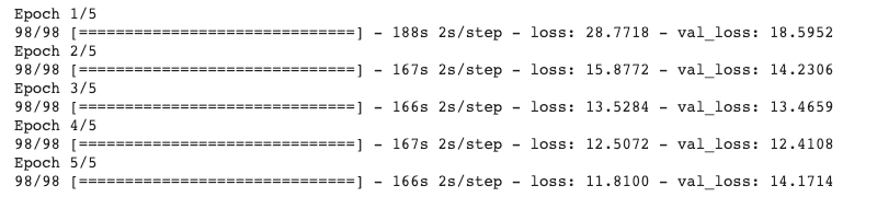
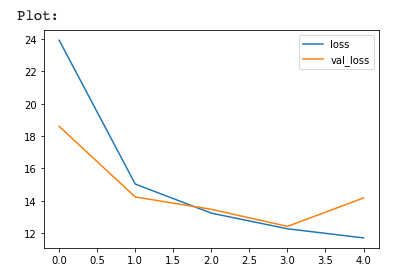
1 | # How did we go? |
1 | import json |
Now let’s use it!
1 | # We can carry these files (*.h5, *.json) somewhere else ... |
Inspect one in detail:
1 | # Encoded image: |
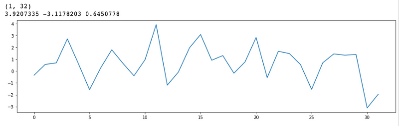
1 | # Latent vector: |
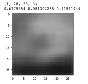
1 | # Reconstructed image |
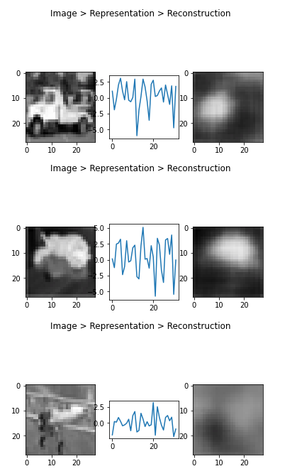
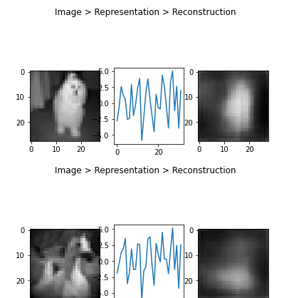
Or in triplets:
1 | def plot_tripple(image, vector, reconstruction): |
1 | x1 = x_test[9] # 2 has a '1', 3 has a '0' |
1 | from random import randrange |
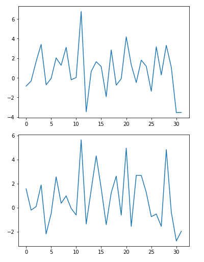
1 | sample_a = x_test[2] # 2 jas a '1' |
z_sample_a_encoded: (1, 32)
z_sample_b_encoded: (1, 32)
1 | plt.plot(z_sample_a_encoded[0]) |
1 | def lerp(u, v, a): |
1 | a = 0.5 |
1 | steps = 5 |
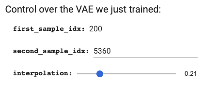
1 | #@title Control over the VAE we just trained: |
Random vector to image
1 | # Random latent |
1 | # We can try break it ... |
Visualization as a gif:
1 | !pip install imageio |
1 | import shutil |
1 | !mkdir images |
1 | interpolate(size = 10) |
1 | from IPython import display |
About this Post
This post is written by Siqi Shu, licensed under CC BY-NC 4.0.