Basic GAN

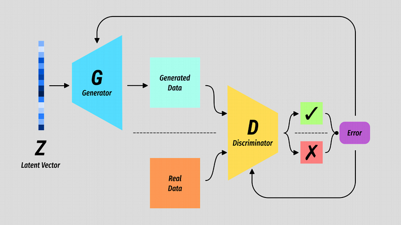
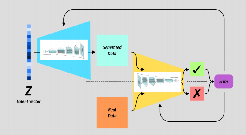
The basic structure of a Generative Adversarial Network.

The Generator G is some kind of generative model which takes a random vector Z as input.

The Discriminator D is a binary classifier which has the simple task of predicting when the data it is seeing is real or not.

The output of D is the value we use to measure the error of both G and D.

Sometimes it helps to view the models separately, and in fact they have no knowledge of one another. All said and done it is the generator that is the interesting bit.

The Training Process

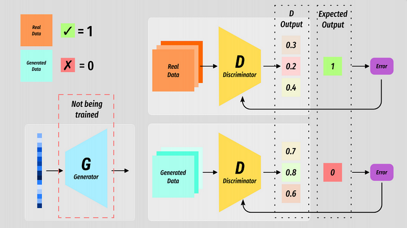
The discriminator(D) is trained in two steps. It is trained in the same way you would train a regular classifier.

A batch of real data is labelled with a 1 and sent through D. D will produce a batch of results and the loss can be measured against the expected label.

A batch of fake data is generated by the generator(G), labelled with a 0 and the process is repeated.

The loss, at this stage, is only used to backprop through the discriminator - G is frozen at this point (no backprop).

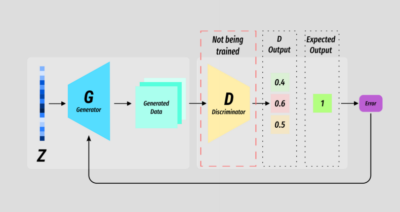
Once D has been trained for k steps (this can vary), we train G for only one.

Again we use the generator to produce a batch of fake data, but this time we label is as real data. This is because we want a measure of how well the generator is doing - we want the generator to produce real looking data.

At this point D is frozen and the error backpropagates through G.

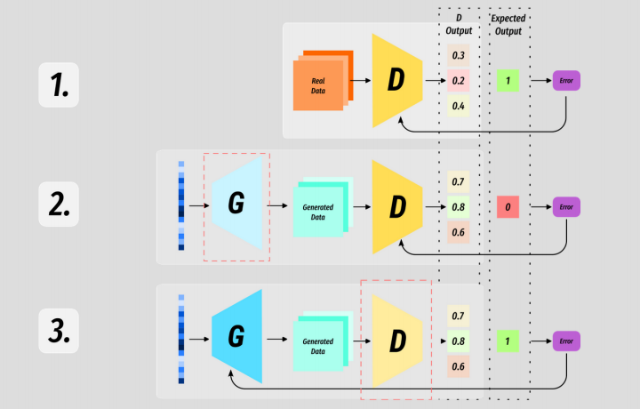
This 3 stage process is the basic training loop of nearly all GANs. In general D is trained on an extra batch than G in order to keep it one step ahead - it is beneficial to keep G playing catch up.

But we will see that there are a huge number of variables and moving parts in GAN training and pretty much every aspect is up for discussion and varies between use cases.

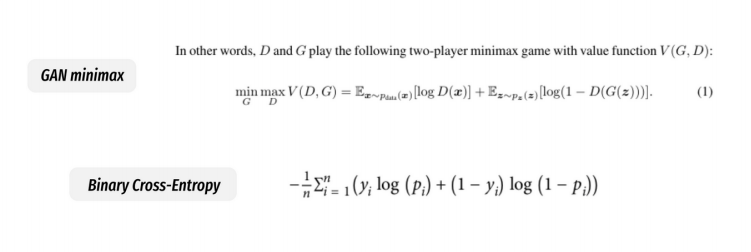
The vanilla loss function looks a lot more complicated than it actually is.

A GAN makes it possible to re-frame an unsupervised learning task into a supervised one by passing all data through the discriminator (a binary classifier). Thus the loss function given in the original paper is essentially binary cross-entropy but re-written.

Goodfellow chose to write the loss function as a minimax value function which makes sense on a high level: there are two players working to outsmart one another.

By inverting a term it allows for a single function which D is trying to maximise while G is trying to minimise. Don’t worry about this too much through, I just think it is good to look at as it is a key part of the original paper.

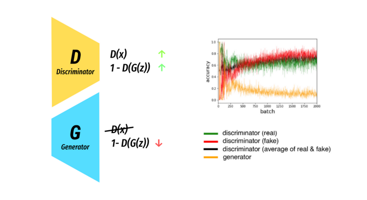
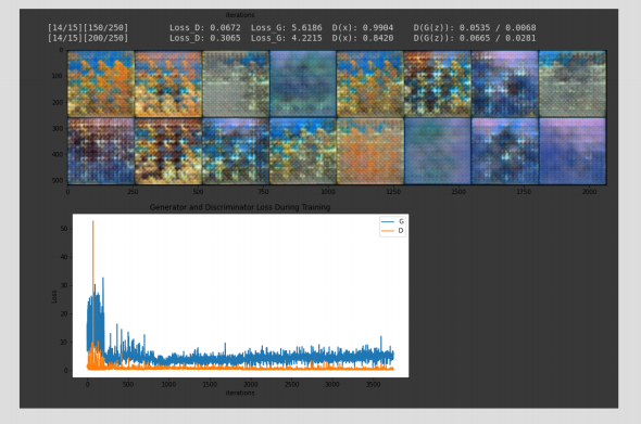
We can see this is practise by looking at the Loss/Time graph of a GAN in training.

Bear-in-mind there a many loss functions and many flavours of GAN! So don’t be alarmed if your GAN loss looks nothing like this.

Training a GAN is a delicate balancing act where the progress of one is based on the other thus gaining a confident measure of progress is difficult.

The loss can be misleading. A generator can be improving in terms of image quality, while the loss can be seen to get worse over time? As with before the loss is measured in terms of the discriminator and so can often be misleading. Giving yourself visual feedback in training is often more useful than graphs.

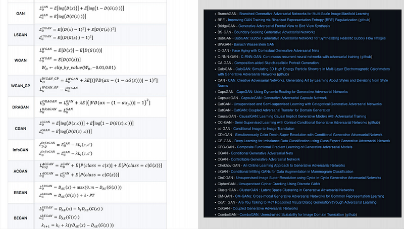
There are a lot of GANs! Finding the optimal cost function/perfect hyper parameters/ the best way of measuring progress of the model is a rich area of research and has lead to a huge number of variants.

Mode Collapse

A failure mode you will no doubt read about is mode collapse/

A ‘mode’ can be thought of as a variant of the training data, if we are training on a dataset of decimal digits(0~9), each digit would be a single mode.

We want G to capture all modes of the dataset. The example image shows mode collapse where the output of the generator is only producing a select few modes.

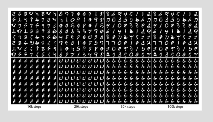
Simply put, this occurs when G gets smarter than D. In practise G finds a particular output which consistently fools D and so learns a mapping of many input Z’s to that output. Remember the objective of G is to convince D that the data it is producing is real so if G finds an output which consisitently fools D and D is unable to learn it’s way out of that trap, G will just keep doing the same thing.

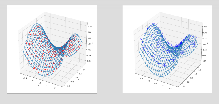
To use our simple GAN from last week, we can see the actual data plot in red dots on the left, and an example of relatively successful training plot in blue crosses on the right. The blue crosses (the output of our trained generator) take the approximate form of the desired data distribution - we are covering many modes of the dataset.

Vanishing Gradients

In the case of vanishing gradients the opposite is true: in this case D has grown too smart too quickly and is consistently assigning the correct label to the data in classification and thus produces has a tiny margin of error.

In simple terms: we want D to be unsure when it sees data produced by G. If it is very confident there error will be close to 0 and thus backpropagation will have little effect as the error is tiny - G can no longer learn!

The image is not the clearest example, but this DCGAN was terminated in training as it failed to improve in the quality of the output. You can see the loss of D is near 0 from early in training.

Wasserstein Loss

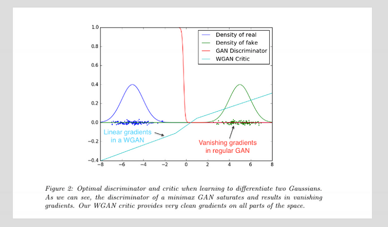
The Wasserstein Loss is an attempt to reframe the loss function of a GAN and has shown to address the failure modes already discussed.

In a Wasserstein GAN the data is now labelled -1 and 1 as labels for fake and real data respectively. We also do away with the sigmoid activation on the final layer of the discriminator meaning the output is now.

For reasons I would do a bad job of explaining this makes the gradients produces by D generally more effective and we are able to train D to an optimal state - we no longer need to worry about it getting too smart.

It is worth at least being aware of Wasserstein Loss as it has led to the Wasserstein GAN-Gradient Penalty framework (WGAN-GP) which can be seen in papers for some common and popular GANs like StyleGAN.

DCGAN

The DCGAN in practice has two opposing CNNs of equivalent structure, but mirror images (aside from the output of D being a single value).

Latent Space Interpolation

Our trained generator G is a function which maps an input Z to an output of the desired shape (some kind of tensor which can be interpreted as an image, sound, text…whatever you’ve trained it to do!).

It follows that changes made to the input Z will berefelcted somehow in the output space.

In literal terms, moving around in space is just a sequence of position vectors.

What if we made a sequence of positions in our latent space and use each one of these Z’s to generate an equivalent G(Z)?

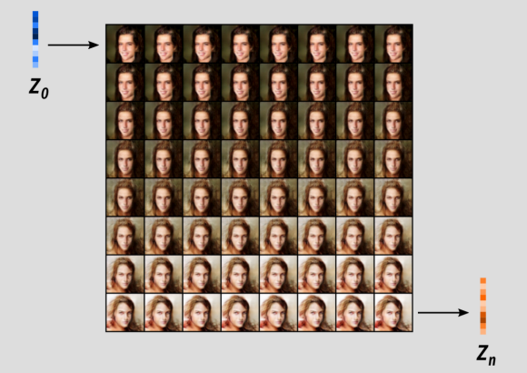
Before we do that I just want to make sure we all understand the word interpolation. So we have an interpolated sequence of latent Z’s/ Now we just take those, one by one, and pass them through our trained G to generate an output! In this instance the model outputs images of human faces.

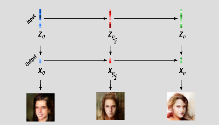
If we increase the number of steps in our interpolation we can see the output is a lot smoother as well! For me this is where the magic of machine learning is. This is so simple but so amazing and mysterious. This is the visual output of simply mapping one space to another: input space to output space.

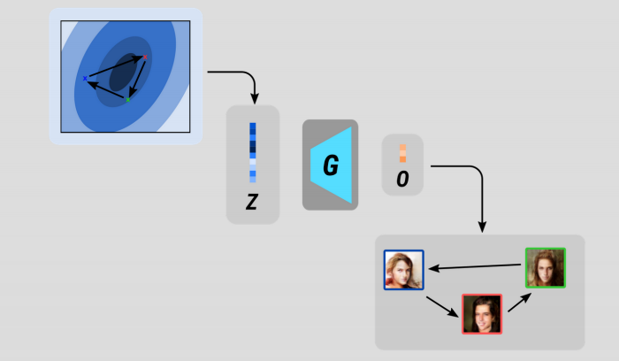
Our way is to search through the latent spce for a specific Z which produce a result close to what we want.

We can treat this as an optimisation task in the same way you would train any other model. But in this instance we are optimizing Z to produce the desired output G(Z).

1. Take a target image.

2. Choose a random Z and get an output image.

3. Measure some error from the output G(Z) and your target image.

4. Backprop the error and adjust Z!

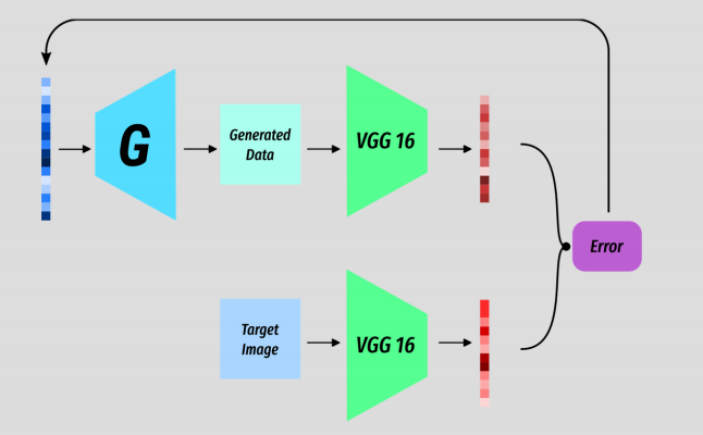
In reality it’s a tiny bit morecomplex as to get some meaningful error we need to run the target and the output through some kind of feature extractor. In the case of StyleGAN they use the classification model VGG16 but only as a feature extractor. But once we have the feature representations of the target and the output we can compute a loss on that and then backprop.