Recap

A look at how we would implement on from scratch in Python.

• Dtaset preparation (including batches)
• Linear Algebra
• Basic introduction to optimising weights

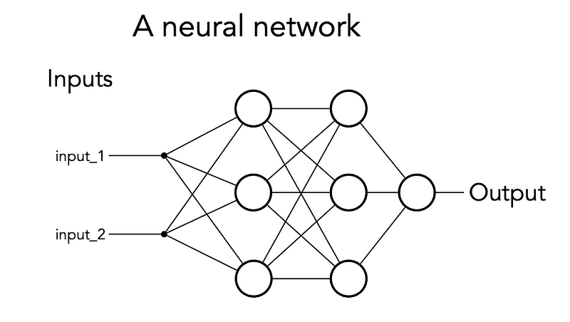
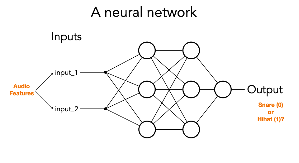
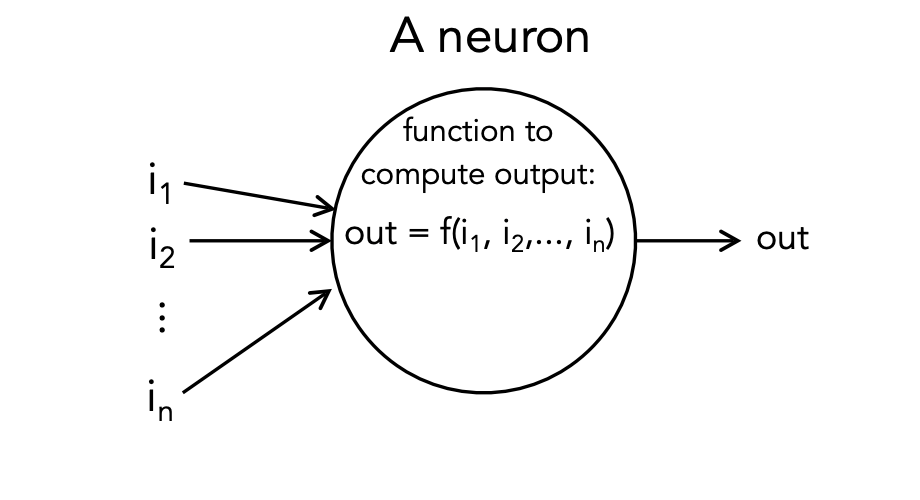
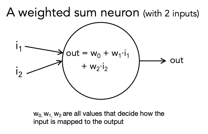
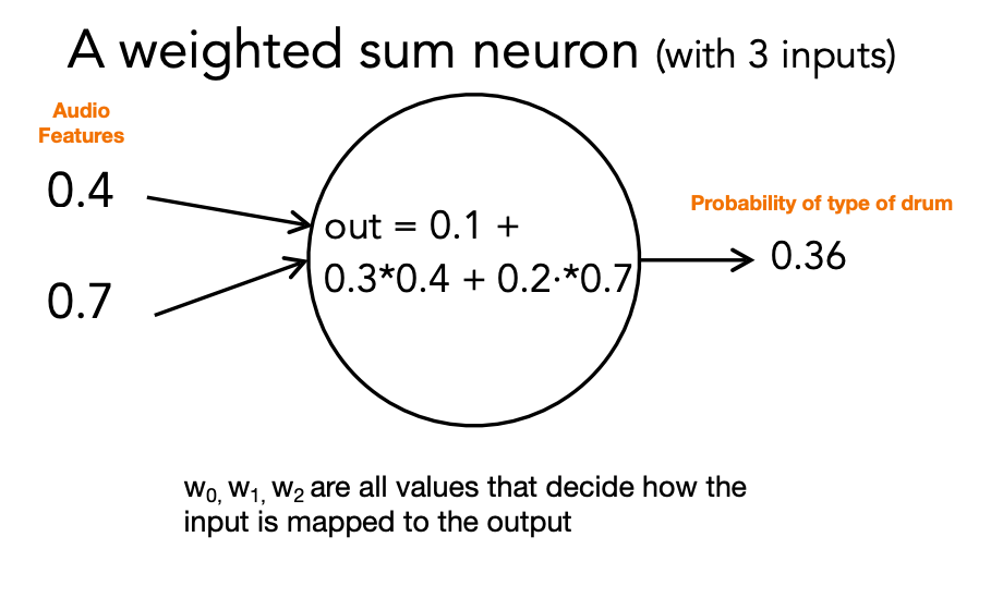
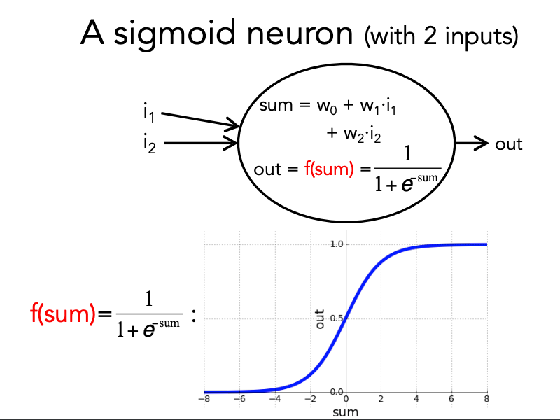
Almost always, we apply an “activation function” to the weighted sum.

Without an explicit function: Neuron outputs the weighted sum.

Alternatively: do some extra computation (the “activation function”) on the weighted sum and output the result of that:

• Inspired by real neurons: fire only when “input” exceed a certain threshold.

In Summary

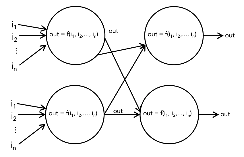
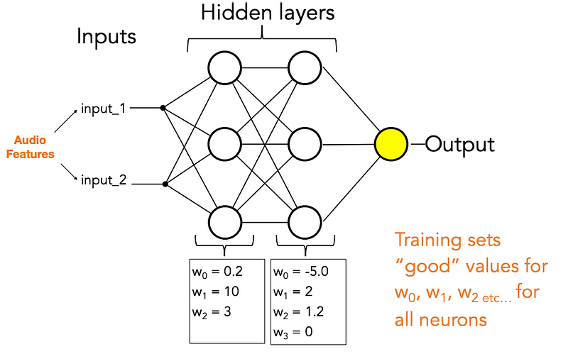
Neural Networks consist of the following components:

• An input layer
• An arbitrary amount of hidden layers
• An output layer
• A set of weights and biases between each layer, W and b
• A choice of activation function for each hidden layer

Loss and Optimisation

How to get your NN to learn the right thing fast?

Loss: what does it mean to learn the “right” thing?

A neural network is a function:

• output = 5 x input + 2

Weights inside each neuron are just numbers that determine what the NN’s function looks like, but good values are unknown in advance.

• output = a x input + b

Training is just the process of finding these good values!

Training examplex are “hints” about what function the neural net should learn.

An very simple untrained NN: output = w1 x input

Training data:
Input Target
3			6
-2		-4
0			0
5			10

What is a good value for w1? How do you know?

w1 = 2 seems to fit this data well.

Linear regression:

y = w1 * X + w0

Which is better and why?

Can we come up with a function (measurement) that gives us better (lower) scores for better lines and worse (higher) scores for worse lines?

Computes a number using only information about:

• The training data targets (“outputs”)
• The neural network’s predicted output values for those targets

Desirable properties:

• A bigger distance between the training data and network output is bad (higher score)
• We generally care about distacne for all examples, on “average”
• We do not care about whether line is above or below an example, only how far it is.

One solution: cost = sum of absolute distances between each example target and the neural network’s output for that example.

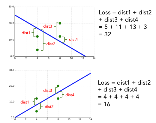
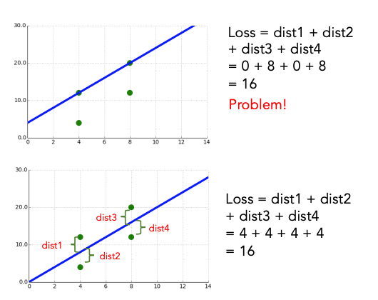
perhaps penalize large distances more harshly than small ones.

Mean-squared error

For each exmaple:

• Compute difference between NN’s predicted output and the training example’s actual target value (i.e., vertical distance between point and line)
• Square this value

Add up the squared difference for all examples.

Loss = (predicted1 - target1) ^2 + (predicted2 - target2)^ 2 + … + (predictedn - targetn)^2

Regression

NN outputs some numeric value between -/+ inf

Mean-squared error (MSE)

Mean squared logarithmic (“log”) error (MSLE)

• First compute the natural log (ln) of the difference between each target/predicted value pair, then compute mean-squared error
• Penalises very large differences less than MSE

Mean absolute error (MAE)

• Our first approach: Doesn’t attempt to overly penalzie large errors at all
• May be better if your data has outliers

Binary classification

Targets are 0 or 1, NN outputs something in (0,1) range.

• Binary cross-entropy loss
  • Summarises average difference between actual and predicted probability distributions for predicting class 1.
  • Treats NN output of 0.95 as “95% certain it’s class 1”; takes this into account when computing loss
• Others exist but not really used for NNs

Multi-class classification

Targets are expressed as 0, 1, … n

NN outputs n values between 0 and 1.

Multi-class cross-entropy loss

• Summarises average difference between actual and predicted probability distributions for all classes
• Use this by default

Sparse multi-class cross-entropy loss

• Same idea, but doesn’t require you to use “one-hot” encoding of each training example.
• Great when you have thousands possible output “classes” (e.g., words in an NLP model!)

KL divergence

• A measure of how different two probability distributions are
• Sometimes used when NN is doing something more complex than multi-class classification (e.g., autoencoder learning a feature representation / embedding)

Resources:

Nice blog post on choosing a loss function -

https://machinelearningmastery.com/how-to-choose-lossfunctions-when-training-deep-learning-neural-networks/

Optimisation

So how do we find good weights?

i.e., how do we find weight values that result in a small loss value?

i.e., what should we know about training so it’s not a mystery, and we have a hope of fixing things if it goes wrong?

A simple example: 1 unknown weight to set

A very simple untrained NN: output = w1 x input

Choose mean-squared error as our loss function.

How does loss change with different values of w1, for a given dataset?

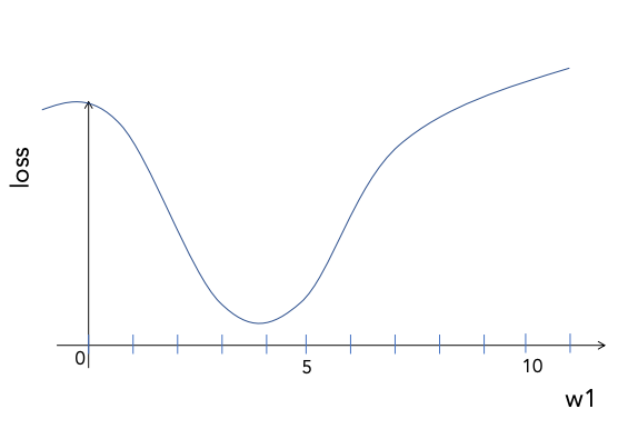
But, we cannot “see” this function directly! We can measure the loss for any given value of w1; we can also compute the slope of the line at any given value of w1, like trying to navigate hilly terrain in a fog; many optimisation methods have been developed for finding good values under such circumstances.

Gradient descent: a simple, standard optimisation method.

1. Pick a random value of w1. Compute loss and slope(gradient) of w1.
2. Pick a new value for w1.
   • Travel “downwards” in slope
   • If slope is steep, take a big hop in that direction. If gradual, take a smaller hop.
   • The “learning rate” of NN is a value between 0.0 and 1.0 that is used to scale these big/small steps.
3. Repeat:
   • For a fixed number of iterations
   • Or until change in loss each iteration is very very small

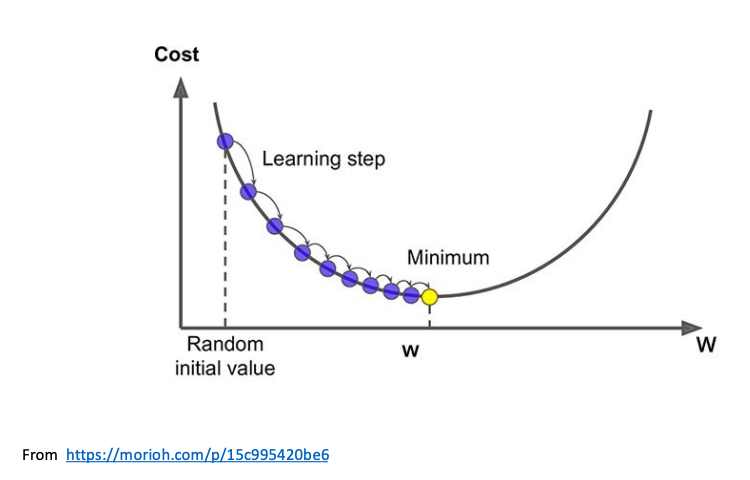
Possible problem #1: Learning rate may be unsuitable

If too small: Takes a looooong time to get to minimum

If too big: Can get lost and never find the minimum

Possible problem #2: Optimization may get stuck in a local minimum

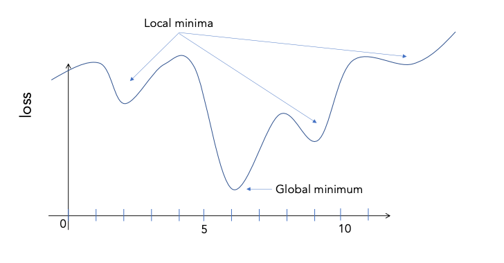
In practice, we always have more than 1 unknown weight, so optimization is finding a minimum in a bumpy surface.

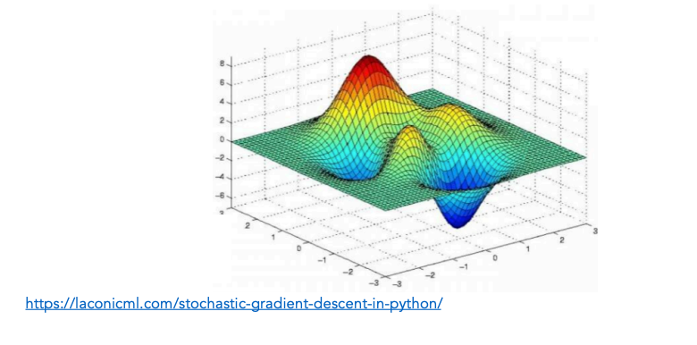
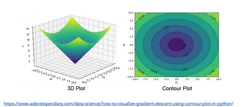
Contour plots: Lines show paths of equal loss

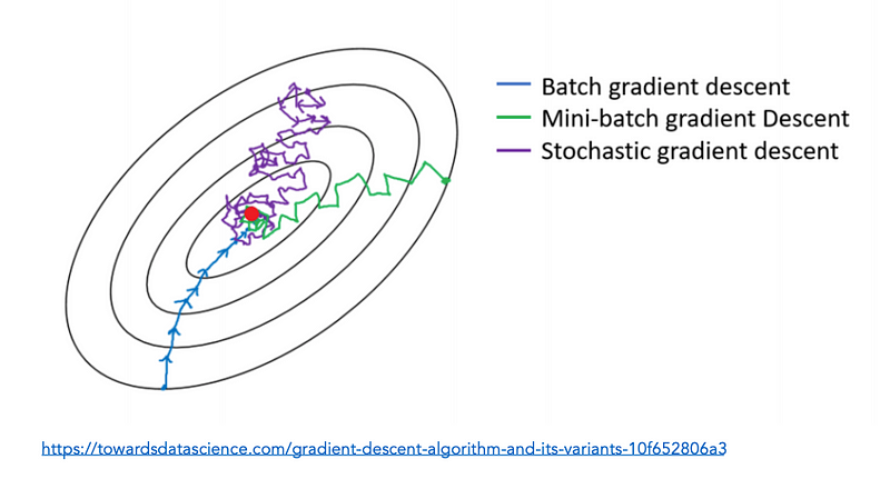
Stochastic gradient descent (SGD) can help avoid local minima (or at least find better local minima).

“Vanilla” (“batch”) gradient descent: use loss computed on all training examples to find the gradient for a particular set of weight values, then follow this gradient downhill.

• Smooth path, but will not “explore” the terrain much.

Stochastic gradient descent: choose a single random example and compute the gradient for a particular set of weight values, then follow this gradient one step. Then choose another single random exmaple and repeat.

• More wiggly path, will explore more terrain over the same number of iterations (but may need more iterations to converge)

Mini-batch gradient descent

A compromise between SGD and vanilla gradient descent: compute gradient at each step using a small number of examples (e.g., 32)

Possible problem #3: Sometimes, it’s hard to find a good set of tradeoffs using the methods we have discussed so far…

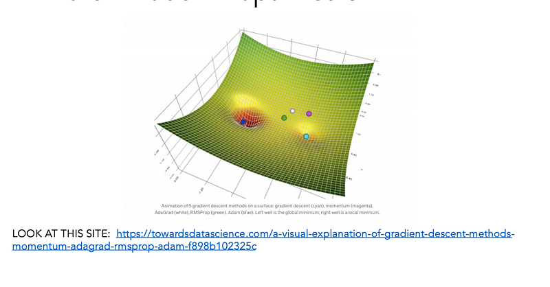
Possible problem #4: The optimal weights might not be so optimal after all

Training finds optimal weight values for the training set.

In the real world, you often want your neural network to perform well on data that isn’t in the training set!

We usually want to “generalise”, not “memorise”.

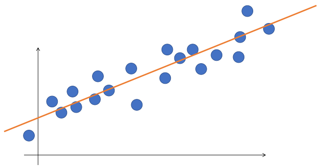
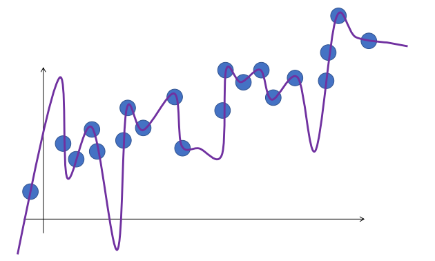
Orange Line has higher loss, but it seems to capture the trend in the data better.

Variation in training examples could be “noise”: maybe we should not try so hard to fit them exactly?

One solution: Regularisation

“Weight” regularisation: loss function includes a penalty for weights that become too large.

Dropout: during training, each neuron “drops out” with some small probability during each epoch. Model is forced to avoid relying too much on particular features.

Another solution: Early stopping

Split the available data into 3 different parts:

• Training set, test set (always use one anyway!), validation set.

Train on the training set

Keep an eye on loss on the validation set

Stop training when loss on the validation set starts to go up

One last trick: Data augmentation

More data is almost always better.

Media data can often be easily “augmented” by introducing random variations during training.

A final detour: Backpropagation

Training a neural network involves:

• Choosing random values for all weights
• Passing some (1/all/some) training examples through the network and computing the loss as well as the gradient of the loss function
• Using information about the current loss & gradient to choose how to change the weights (i.e., a “direction” and an “amount” for each weight)
• Different optimisation methods will use loss function value & gradient in slightly different ways to try to get to a good set of weights
• Backpropogation: this is the algorithm for computing the gradient of the loss function.

Why is backpropagation cool & important?

Taking a purely mathematical approach to computing gradient is slooow.

Back-propagation is more efficient (fewer # of computational steps, less time in practice)

• Gradient for final layer of weights is computed first
• Parts of this computation are used to compute the gradient for weights in the previous layer
• And so on

General tips for making NNs that work

1. Start with mean-squared error for regression, cross-entropy loss for classification unless you have a reason not to
   • E.g., you are using a research paper or existing implementation that uses something else.
2. Start with adam optimiser unless you have a reason not to
3. Sanity check throughout:
   • Keep an eye on your loss through each training epoch
   • Examine your data (visualize it, look at examples that are misclassified, etc.)
   • Try training on a really small version of your dataset and make sure you can overfit (if not, something is wrong!)
4. When things do not work, try changing: your data, your features, data augmentation, your network architecture, your loss function, your activation function, regularization, your optimizer, your optimizer parameters.
5. Use a validation dataset for early stopping if you can, and only trust your held-out test set (if that) to indicate how well your trained model may work on new data.

Finasl notes

1. Even experts do not always know waht the “best” loss functio nor optimizer is.

2. ML involves a lot of experimentation:

   • Some tools can make this easier, e.g., Kera Tuner
   • You can also make this easier by keeping track of your results, using visualisations and sanity checks frequently, etc.

3. You do not need to make perfect decisions, only reasonably good ones.

   • Choice and processing of training data, choice of model type, choice of learning problem are all likely to have big impacts.

4. Loss is only a number

   • What really matters is how well your model works in teh “real world”

Other resources

Great tutorial with visualisations for different optimization methods

https://towardsdatascience.com/a-visual-explanation-of-gradient-descent-methods-momentum-adagrad-rmsprop-adam-f898b102325c

Great video going into more detail about gradient descent, in general:

https://www.youtube.com/watch?v=IHZwWFHWa-w

Great video from the same source about how gradient descent relates to back- propagation

https://www.youtube.com/watch?v=Ilg3gGewQ5U&list=PLZHQObOWTQDNU6R1_67000Dx_ZCJB-3pi&index=3

Nice blog post on gradient descent

https://towardsdatascience.com/gradient-descent-algorithm-and-its-variants-10f652806a3

Another blog post, comparing gradient descent, SGD, and mini-batch:

https://machinelearningmastery.com/gentle-introduction-mini-batch-gradient-descent-configure-batch-size/

General deep learning practical tricks summary

https://stanford.edu/~shervine/teaching/cs-230/cheatsheet-deep-learning-tips-and-tricks