Audio basics

Audio waveforms are lists of amplitude measurements than can be used to control the positions of a speaker in order to recreate observed pressure fluctuations.

They are generated by microphones by suspending a small filament of conductive material in an electromagnetic field and measuring its motion as sound passes over it.

You can also create them synthetically (e.g. with a sin function).

Usually we need to record 44,100 audio amplitude measurements each second in order to be able to reproduce sounds roughly the way we hear them.

Actually the number is sort of arbitrary as long as it’s more than twice the human hearing range (20,000 Hz as a rough max).

We usually store each of these amplitude values as a 16 bit value (as a minimum resolution).

This is why audio waveforms are usually lists of 16 or 32 bit values. They go between -1 and 1. This represents a normal range of speaker motion. When the speaker is moving out, the values are increasing above 0 to a maximum of 1, and when the speaker is moving in, it;s decreasing to a minimum of -1. However, -1 is just as ‘loud’ as 1 in these situations, as waveforms are bipolar and oscillate around 0.

What is an Audio Feature?

A form of information that you canderive from audio data that tells you something specific about the audio recording.

• E.g. how loud it is, where events might be, how noisy it is, if there are any musical features(pitches, sound types).

Audio Buffer

It’s common to use a short slice of audio data when generating or analysing audio signals. For example, when playing back a sound, you do not need to load the whole sound in to memory - you can just grab a short section. This is called ‘buffering’, and it’s used all the time in real-time audio. It’s cool because we can go through the audio in small chunks whilst we are listening to it, and graph the output at the same time. Otherwise we’d have to load the whole thing in and then wait for it to be processed before we can see it. This is cool for some things (and can actually be better), but it is less flexible.

Getting Information out of Audio Buffers

You can get information from an Audio Buffer very easily:

• You can just take a few values and try to understand what they mean
• Or you can take the whole buffer and compute basic stats on them.

The easiest thing to do is compute the average amplitude value, the peak amplitude value and the minimum amplitude value in the buffer. We are going to write an algorithm to get its average, minimum and maximum values.

// assuming audioBuffer contains the audio buffer values
// and that bufferSize is the same as the number of values in the buffer

let avg = 0;
for (let i = 0; i < bufferSize; i++) {
  avg = avg + audioBuffer[i];
}
avg = avg / bufferSize;
console.log(avg);

// assuming audioBuffer contains the audio buffer values
// and that bufferSize is the same as the number of values in the buffer

let peak = 0;
for (let i = 0; i < bufferSize; i++) {
  let currentAmp = Math.abs(audioBuffer[i]);
  if (currentAmpt > peak) {
    peak = currentAmp;
  }
}
console.log(peak);

// assuming audioBuffer contains the audio buffer values
// and that bufferSize is the same as the number of values in the buffer

let minimum = 0;
for (let i = 0; i < bufferSize; i++) {
  let currentAmp = Math.abs(audioBuffer[i]);
  if (currentAmpt < minimum) {
    minimum = currentAmp;
  }
}
console.log(minimum);

Looking for events

So far the stats we have talked about ahve mainly told us about how loud things are in different ways.

We can use them to check the level of a signal, and probably control animations etc.

If the values in the audioBuffer cross a threshold value:

• e.g. > 0.5 this might be an indication that an event has happened.

But they also might be random fluctuations. We could use the average of the values in a chunk of audio to smooth the signal, and then test to see if the average value is over a certain amount. If it is, we could do something, like draw a box, or drop a maker. It is not very accurate, but it kind of works.

It is better if we do not smooth as we get a better measure of when thing actually happened. Butthis creates other problems. For example, what happens if we detect an event, and then the value of the audio waveform stays high or goes higher? We will get lots of false positives. This is common because a sound might start, and then get louder, but still be part of the same event.

What might we do to mitigate this?

• Solution 1: wait for the audio output todrop below a threshold before we allow it to go looking for new events.
• Solution 2: set an amount of time that is the minimum duration between events - e.g. when an event is detected, start counting and do not allow any more events to be detected. After you have counted to a specific value, start looking for events again.

One of the major issues here is that there are changes in audio that might be important, but that are not necessarily reflected in the amplitude values very strongly.

A musical melody might have lots of different pitches in it, but they might not look any different in terms of amplitude (unless they naturally have gaps between them).

So, importantly, what kind of information is this, and how can we go about finding it in the signal?

There are lots of ways of trying to extract frequency information from an audio buffer. The most important method is known as the Fourier ransform.

The fourier transform can tell you a lot about the universe, and provide you with spectral decompositions. The maths behind the transform are a bit off-topic for this session (I can point you at some details if you are interested).

But it is much more important to understand what information comes out of the Fourier transform, and how to create it!

What goes in, what comes out, and in what form

There’s a version of the Fourier Transform that is really efficient for real-time use, and it is called a Fast Fourier Transform.

It is useful because it provides us with lots of great information very quickly by only using a block size that is a power of 2.

This is cool because our audio blocksizes are usually also a power of 2. So we can just take our audio buffer and stick the whole thing in an FFT buffer.

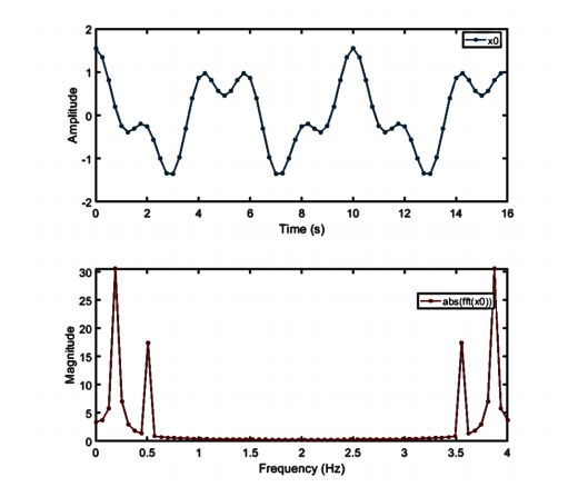
It then gives us back a whole bunch of information about how the amplitude values intersect with sin and cosine waves over a range of different frequencies - thus giving us some idea what kind of frequencies are present in the data.

The engineering behind how this works has lots of problems, for example: what happens if your audio buffer has lots of waveforms in it that are halfway through their period? Nasty.

In this case, we crossfade FFT buffers together in an ‘overlap-add’ process to reduce discontinuities. The more we do this, the better the result but this is not necessarily that important in information retrieval.

Also, the FFT produces twice as much data as you put in. This is pretty simple but not that important here because for most of things we are going to do, we won’t need all of it and we can simply throw it away.

What we need to know for now is that each pair of output values in the FFT array is the amount of energy in each frequency band expressed as two numbers - a complex number that represents a position on a 2D graph which you can think about as an x,y Cartesian plane - although it is considered a complex plane.

If we want to get the energy in each of these bands, we can do this by converting these two values (x,y) into a single magnitude value using a Pythagorean approach -x^2 + y^2 = mag^2.

The output of this is a simgple value which contains just the energy in each band.

The even better news is that we only actually need half of this data - the first half of the array. So we can throw the other half away.

We call this a real FFT, or rFFT. Most of what we are going to do only needs the rFFT. It is half the size of the data we put in, and a quarter of the size.

SO what does each value in a real FFT (rFFT) really mean?

well, given a samplerate of 44100, you can get the width of each band by dividing 44100 by the size of the audio buffer.

This is also known as the Bin Frequency. Each value in the array (number in the list) represents energy in a specific bandwidth equal to the bin frequency.

So in real terms, with a samplerate of 44100, and an FFT size of 1024, your bin frequency is 44100/1024 = 43.06640625Hz.

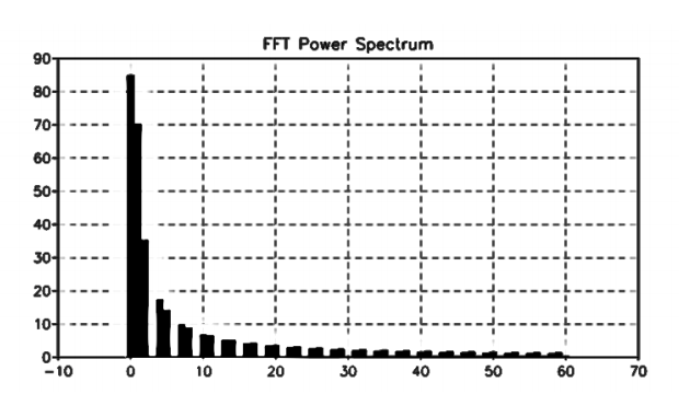
You might notice that half the FFT rate, the bin frequency is > 22050, which is why we only need half the data. The second half of the output is actually just a mirror image of what you will find in first half, which is why we do not need it.

FFT statistics

SO we have an array of values that tell you what spectral energy is in a chunk of audio. It can tell you about the frequency distribution of the waveforms in the signal. We can use this to create an audio ‘fingerprint’ of any sound. Most FFT frames are less similar than you think.

So once we have the list of values, we can do the same things with it that we just talked about:

• We can get the average, the lowest val, the highest val, the standard deviation.

• We can get the absolute difference between consecutive frames, and then get the average of this difference. This is called ‘spectral FLUX’. It is great because it can be used to capture note events, as note events are often changes in frequency.

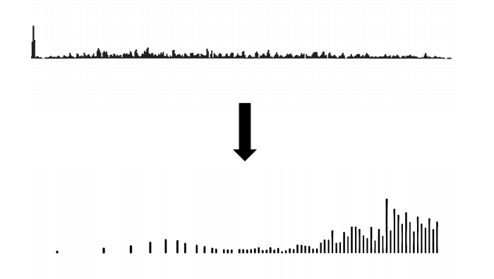
FFTs are great, but they do have a couple of issues. The FFT gives us a linear output, meaning that doublings of frequency are spread futher and further apart in the data. This is not how we usually hear sounds. If we double the frequency of a musical note, we hear it as octave up, and to us, and octave is not much. If we double it again, we also hear it a further octave up - the smae distance, and we recognize it as the same note. But in the FFT they are represented further apart each time.

CQT

The constant Q transform (CQT) takes the FFT and reduces it to a much smaller number of values, like say, 128.

We don’t need to know precisely how this happens. Yes it is a loop, we need to take energy from some of thebins and stick it in fewer bins, we need to have a rationale of how and hwy to do this.

Usually the rationale used is octaves, where Q is thebandwidth in ‘logaritmic’ frequency, so that an octave is spaced out evenly across the bins.

MFCC

This is the best audio feature if you want to create a small audio fingerprint.

We can take a CQT and then do a consine transform on it (half an FFT). This will give us a msall ‘spectrum of a spectrum’.

Also called CEPSTRUM, this can be much smaller than an FFT (as small as 12 numbers) and be much better in some ways:

• More robust to noise and amplitude variations.
• Easier to store and access
• Quicker to search through

If we convert a bunch of FFT frames to cepstrum frames, this is a great way of matching audio!

FFT / MFCC visualiser https://mimicproject.com/code/ee2fbb9e-f474-fb4e-033d-7453fd05c043

MFCC Classifier Demo https://mimicproject.com/code/3864f3e5-8263-b70e-5ef9-1037c724d4ec

MFCC -> Learner.js – great example to build on https://mimicproject.com/code/7b2ab7db-77a2-ce81-da66-d805126098c6