In this article, we will look at how to predict discrete labels.

Predicting Discrete Labels

Our intention is to make a model that generalises to a problem well, so that when it sees new data, it will predict the correct labels.

Evaluating Classifiers

Overfitting - when the model fits to exactly to our dataset and doesn’t generalise to the problem well. This will perform badly on new data. Characterised, but low test set accuracy.

Underfitting - when a model has failed to fit the necessary complexities of the data and problem. Characterised by low accuracy in general.

K Nearest Neighbour

This simple classification algorithm is actually the one we used on MIMIC project with the Learner.js library. There is not even technically any training with this algorithm, the dataset is the model.

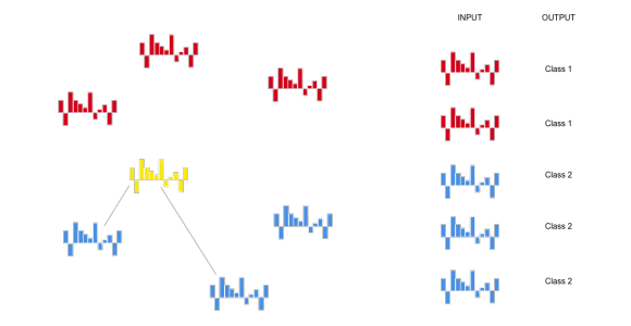
Predicting a new label

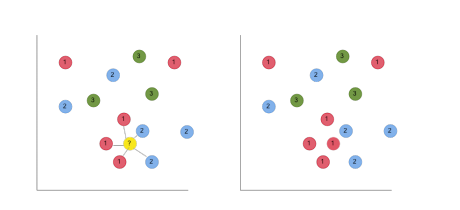
When we get a new data point to classify, we simply predict the label of the nearest example in the dataset; if k = 1, this is the single nearsest.

When we get a new data point to classify, we simply predict the label of the nearest example in the dataset; if k = 5, this is the most frequent of the 5 nearest.

Euclidean distance

To find the nearest neighbours, we take the Euclidean distance, this is done using Pythagoras Theorem.

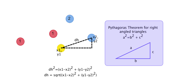
This works in more than 2 dimensions, so we can use this no matter how many features we have.

Why change K?

Imagine we have a dataset collected with a proximity sensor that records how near art gallery visitors are to our smart machine installation lighting experiences.

We have used a KNN classifier to model people’s habaviour around it, and change to different lighting patterns depending on what class the model has predicted.

Mostly the sensor is pretty accurate at telling us where visitors are, but about 10% of the time it fails to measure correctly and gives us what is essentially a random number.

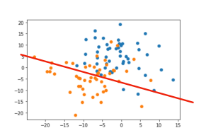
Noise in the data

Our feature representation and dataset is actually good, so there should be two distinct groups, however, the noise has muddled the groups a bit.

We know the behavior we want the model to capture is less intermingled (closer to the red line); this is sometimes called irreducible error.

Decision Boundary

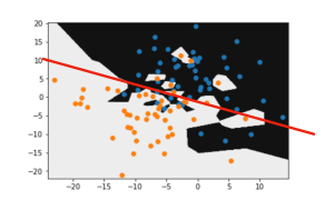
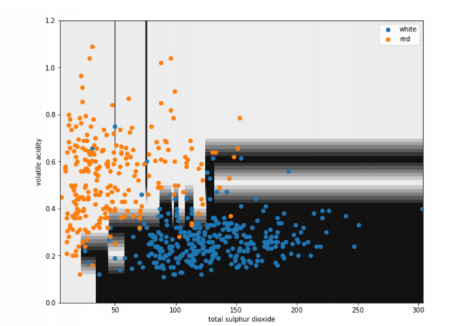
We show the dataset here, with a decision boundary. This shows us the classes that would be predicted for a wide range of values.

With k = 1, there are lots of small pockets of each class as the classifier responds to the noise because even one bad piece of data can throw off the classifier.

This is a danger of overfitting the data.

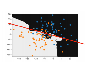
With k = 5, the boundary begins to smooth out.

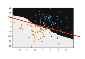
With the k = 20, the boundary now looks like how we know we want our model to bah, with the noise in the dataset not having as much influence.

We can now use this model to accurately predict visitors behavior in the installation and provide appropriate response.

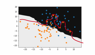
However, if in fact the phenomena we are trying to model actually has this complex shape and variation, having a high k value will smooth over all this variation we actually want in the model.

This would be a case of underfitting, and we would model error is down to high bias.

Relation ships are not alwat simple or linear, and one of the advantages of KNN is it can fit very comple decision boundaries.

Ocam’s Razor

Ocam’s Razor tells us to pick the simplest solution our evidence suggests. If we have enough data, we can justify a complex decision boundary (left).

If not, weshould favour a simpler model (centre).

We would say the model on the right has high variance, in that small changes in the training set result in large changes to the model.

Decision Trees

What is decision trees?

A series of binary choices, model trained to 93% accuracy.

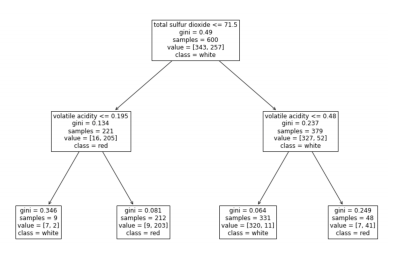
We. Start at the root node, leaf nodes determine a final choice.

Clearly show decisions made by each block.

Gini Impurity

Each node tells us how many samples in the training set belong to each class at that point. It also tells us the “GIni Impurity”. This is a measure of the ratio of training instances for that node.

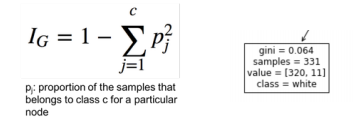
1 - ((320/331)^2 + (11/331)^2) = 0.064

If Gini Impurity is 0, then the all the training examples in that leaf node are of the same class and the node is “pure”.

In general, the lower impurity, the better the prediction is at that node.

Unlike some models, Decision Trees are considered white box, in that we can look inside and watch every once the model has made to arrive at its prediction. This is in comparison to black box models like Neural Networks.

Training

We will use the CART algorithm.

When we are “growing” the tree, we pick a feature (e.g. total sulphur dioxide) and a threshold (e.g. <= 71.5) for the new node.

Unsurprisingly, we aim to minimise the gini impurity when training.

Left=9/221 samples, Gini=0.346

Right=212/221 samples, Gini=0.081

CART cost function:

• (9/221 * 0.346) + (212/221 * 0.081)

High impurity has less of a impact on the cost if the amount of training data in that node after the split is a small proportion.

We keep going recursively splitting until we reach the maximum specified depth or the best split we can do doesn’t reduce the cost function.

Reducing Overfitting

We have seen that with a model that has max_depth = 2, we can clearly see the two decision boundaries. If we increase the max_depth, we get a more complex model with more choices, and a more complex decision boundary.

For the same reasons as with changing the k value in KNNs, we should only have a model that is as complicated as we as need. This really looks like it has overfit to the data, and the lower depth makes a simpler model that will generalise better.

Random Forest

Bagging Decision Trees

Random Forests train mutiple Decision Trees at once.

We then pick the most common prediction out all of them.

We can do this with any types of classifiers, and its known bagging.

For Random Forests, each tree is trained on a different subset of features, meaning that when we ahve averaged all the results across we are likely to get a better, more robust result.

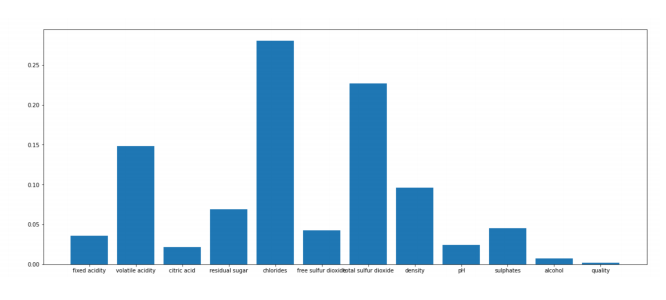
It can also show feature importance, as we know which features were involved in the trees that contributed to correct results. A Random Forest with all 12 features gets 99.2% test set accuracy.

This graph shows feature importance and that chlorides and total sulphur dioxide are in fact the biggest contributors to this models performance.

Interestingly, quality scores are the least important to predicting whether a wine is white or red.

Summary

Both KNN and Decision Trees are capable of fitting complex decision boundaries. But this might cause overfitting, depending on the complexity of your problem, and the amount and quality of your data. You can reduce this by restricting the complexity of the models, but be careful not to underfoot. These are issues for both regression and classification tasks.